Controls Theory

Nov 25 2021

Control theory is a branch of mathematics and engineering, which defines the conditions needed for a system to maintain a controlled output in the face of input variation. In simple terms, we seek to stabilize our system through some control theory concepts when many factors can destabilize it. At the end of reading this article, you can expect to have an overview of control theory with some basic knowledge of PID control.

To understand this, first, let us know a few terms:

1. Input: The set of instructions given to the system

2. Output: Consists of a group of variables that describe the state of the system. Usually represented by 𝑥

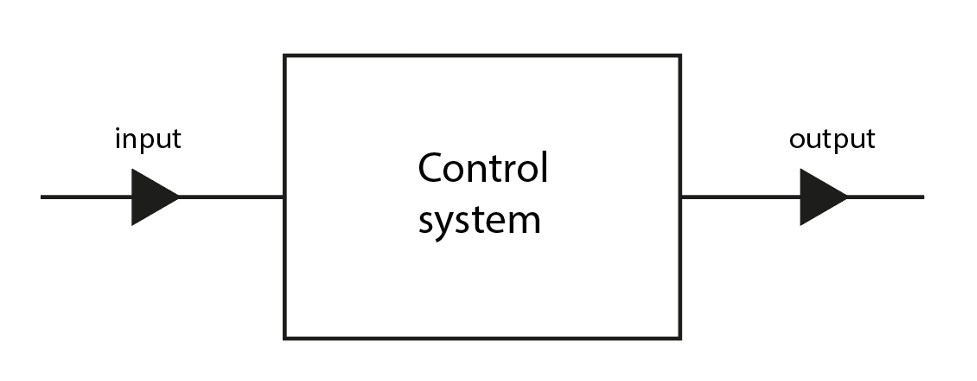
3. Control System: The entire system, which includes a controller, plant, and sensors, is collectively known as a control system. The plant is a part that is controlled. The controller provides control commands to the plant. Sensors measure the state of the system. See the flow diagram for reference:

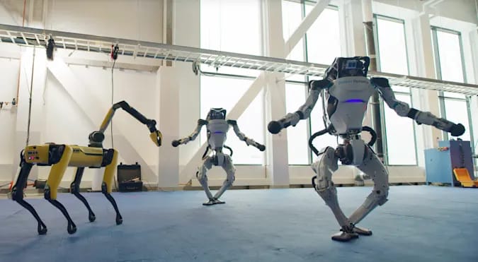
To put these terms into an application, let’s take the example of a person driving a car. (Pause here and try to identify what could be the input, output, and control system in this example.) So, in this case, the input could be instructions given to the driver by his brain. The driver will be the controller, which controls the car using the instructions received. The vehicle will be the plant; sensors would be the speedometer, driver’s eyes to see the traffic, ears to listen to any horn, etc. The output could be the velocity of the car, current traffic conditions on the road, etc.

Now that you understand basic terms let's move on to classifying control systems.

We classify control systems on various bases, but the most prominent ones are:

1. Based on feedback (output)

Open-loop control system - In this type of system, the input given to the controller is independent of the output. In the above car example, we can see that if the driver doesn’t pay heed to the current state of the system(the output) and drives it just based on some pre-learned instructions, then this system would be an open loop, as there are no changes made to the input depending on the output. As you must have noticed, this type of system is problematic as it cannot account for any uncertainties.
Closed-loop control system - Here, the input commands are based on the output received. For example, when a car stops in front, the driver’s input will change, and they will apply brakes.

2. Based on energy expenditure

Active - In this type, a certain amount of energy is required to implement the control commands. For example, to accelerate the car, it will consume fuel.
Passive - This system involves minimal energy expenditure to implement the input into the system. For example, if the car goes downhill, it can be controlled by just applying the brakes.

Since we now have an overview of control theory, let us bring some maths into the picture, let the input function be u(t) and output function be x(t).

Wondering what use maths is of? Read on...

Control Law

Various types of systems have different anomalies present in them. In many cases, we can express the output and correction to the input to control the system through some mathematical relation. This relation is known as a control law. So, a control law is a mathematical law that relates output and input, along with other control command parameters or measurable properties of the state.

Example: u(t) = -K(x(t) - x0)

There are various control laws, such as Linear Quadratic Regulator (the above example is an LQR), PID control, etc., which may be helpful in different scenarios. One such law is PID which is widely used even in industries because it is simple and works for almost every case.

Proportional-Integral-Derivative (PID)

The control law for PID is:

Don’t get overwhelmed with the equation! It’s pretty simple when you understand it.

Let us understand what each term is:

1. Kp is the proportional coefficient/weight

2. Kd is the derivative coefficient/weight

3. Ki is the integral coefficient/weight

4. Ti is the integral time constant

5. Td is the derivative time constant

Here, e(t) is the error between the desired and the actual state.

This law has three parts: proportional, integral and derivative parts; each one of them has its own importance.

Proportional(P)

In this the input is linearly proportional to the error, which means that the error is just scaled using the constant Kp.

Integral(I)

The integral of error over time is scaled with a constant Ki.

Derivative(D)

Here, the derivative of the error is scaled and multiplied by the constant Kd.

Each of the above components aims to correct different causes of the error, and together these three combine to give us the best desired output.

Let’s understand the use of all the above three components using an example of a self-driving car. We have to design the controls of the vehicle. The car is supposed to move on a given marked line. Let's start with our analysis:

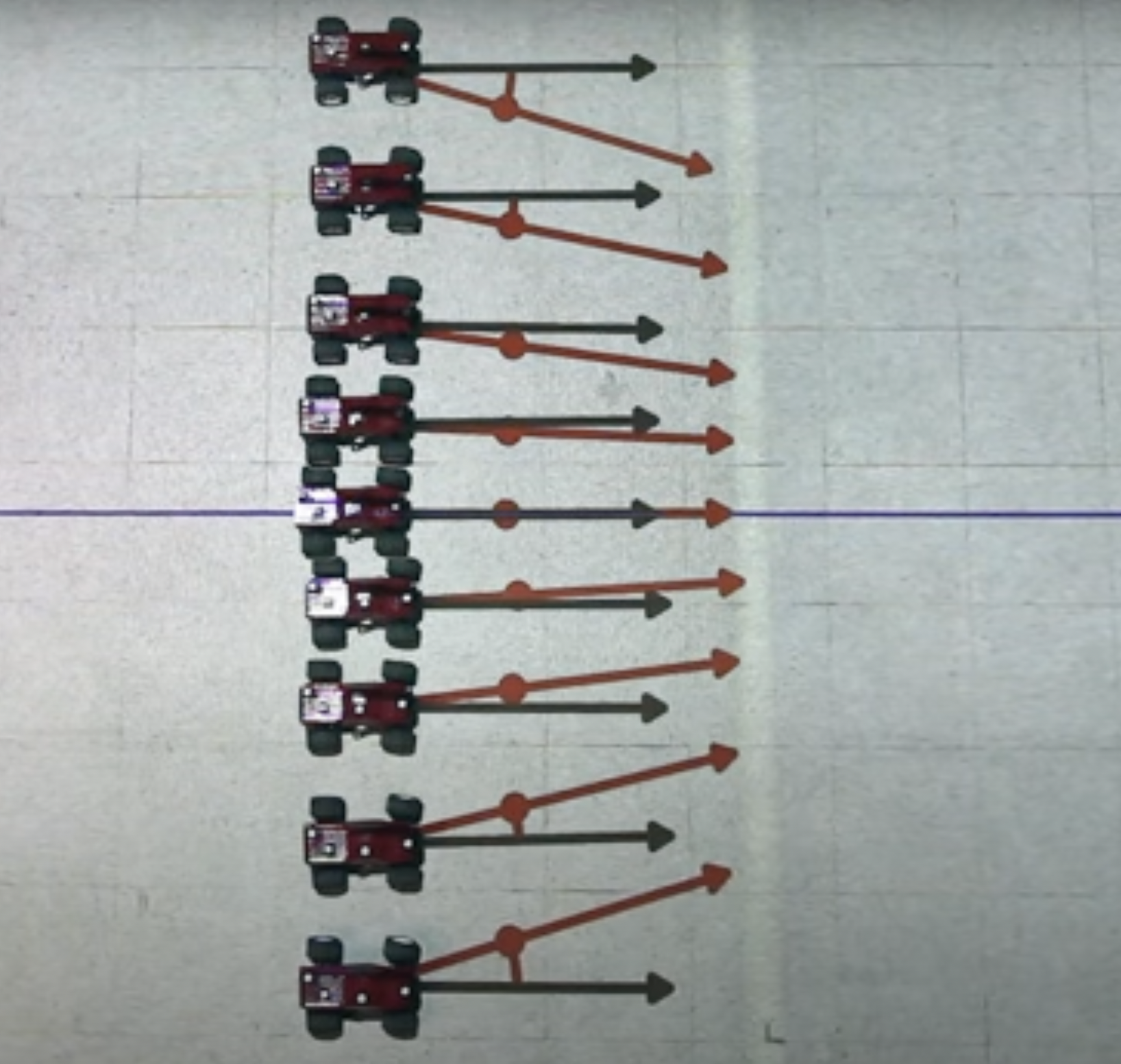
The input given to the car is to turn its steering wheel to left or right by a fixed angle, as shown below.

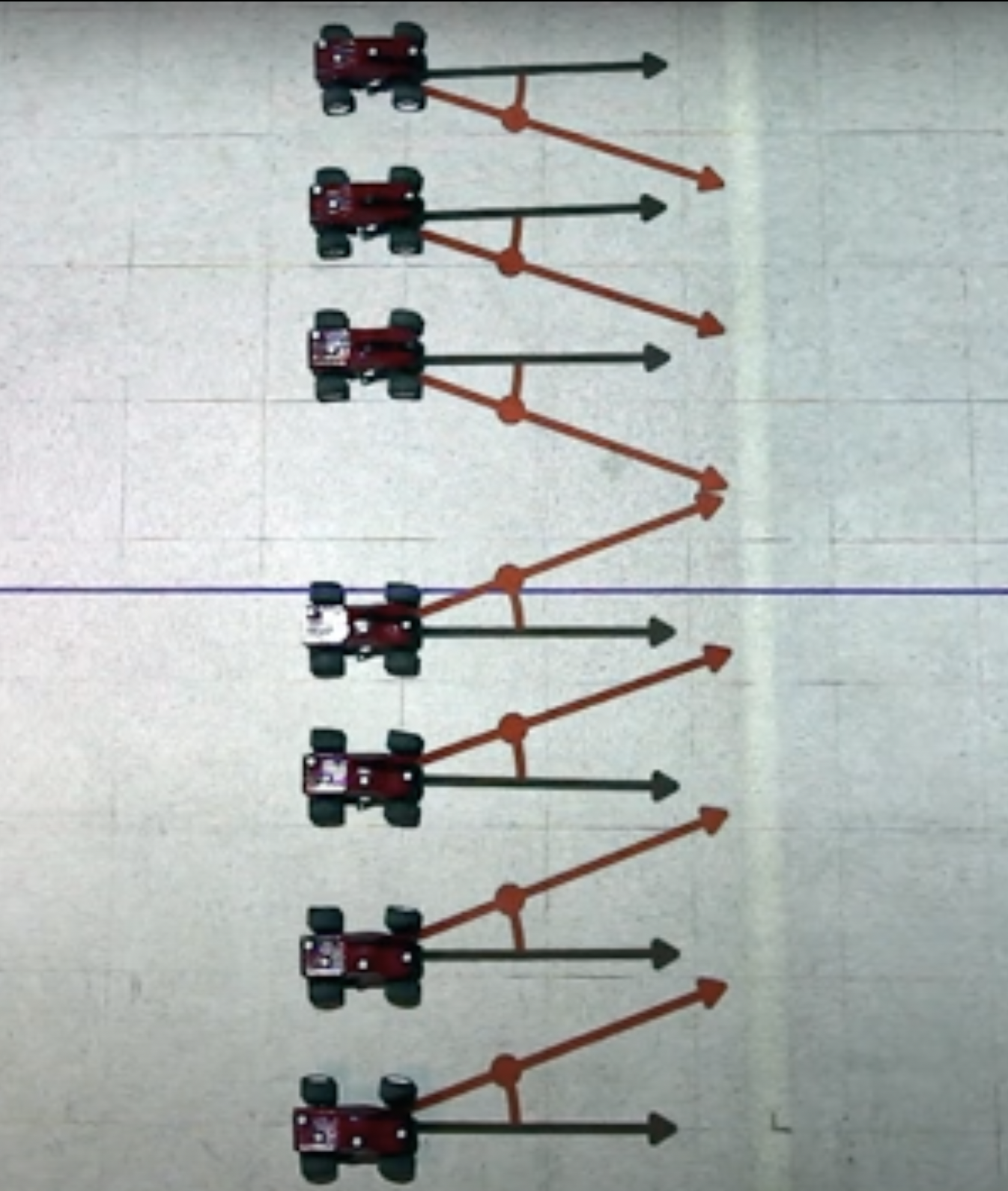
But there is a problem with this; we are instructing to turn the steering wheel by the same angle even if the car is slightly offset. This will make the vehicle constantly oscillate around the line, and the ride will be jerky, making it uncomfortable for the passengers.

So what can be done to solve this? We need to turn the steering wheel in proportion to the error, i.e., its offset from the line. This is where the P part comes into play. Notice what will happen if we give the input as: u(t) = Kp e(t)

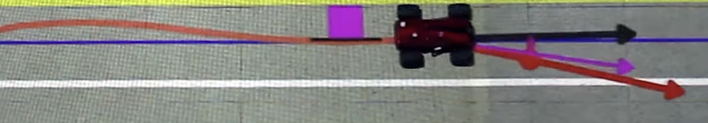
Here we turn the steering by a smaller angle if the error is small and the problem is solved. But there is a problem with this too! This control works well with low offset, but it may lead to a situation like below when the error is high.

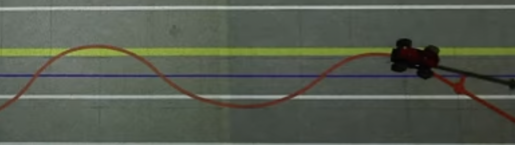
Since the initial angle is high, the steering angle is relatively high, but as a result, it leads to the car closing in on the line much quicker, even quicker than what the car can account for by decreasing the angle; hence it will overshoot. And again, the same story will repeat from the other side, leading to oscillations.

So how do we solve this? Here’s where the D part comes in handy. The input is modified as: u(t) = Kp e(t) + Kd e'(t)

The added term takes into account the rate of change of error. So if the error is decreasing rapidly, e'(t) will be highly negative. So when the error is enormous, the proportional part will be high, but as the car starts to steer, the derivative term will increase in the negative direction, avoiding the car to turn too quickly. So we will get an ideal situation as below:

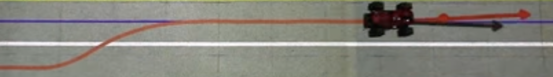
This is collectively known as PD control.

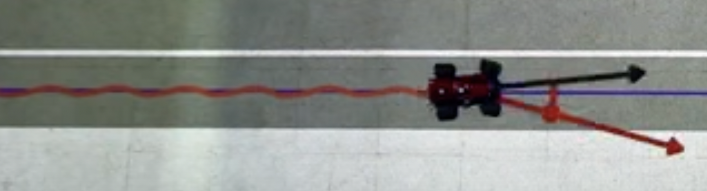
Wait! There is still a problem. Only P and D can lead to an error known as steady-state error. Take the following case: Let's say the car is driving at a small constant error parallel to the marked line (purple).

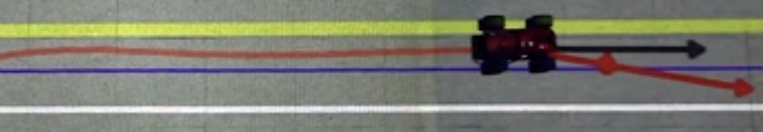
How will the P and D act in this case? Since the error is small, the proportional part will steer through a slight angle, but as soon as it starts turning, e'(t) will become negative and nullify the P term; hence the car will continue with a constant error (steady-state error).

The I part helps to account for this error. The input function now becomes:

u(t) = Kp e(t) + Kd e'(t) + Ki ∫e(t).dt

Integral term adds the net error till the current time and tries to make it zero.

So here, the integral part will add up the steady-state error and slowly reduce the error.

As we can see from the above image, the initial small steady-state error is quickly reduced to zero using the Integral term.

This completes our analysis of the PID control law. Note that the constants Kp, Kd & Ki are tuned ample times to get the perfect combination of the three, such that none of them overshadows the other terms, and we get our desired output.